Introduction
Once a genome has been assembled, it is important to assess the quality of the assembly, and in the first instance, this quality control (QC) can be achieved using the workflow described here.
Figure 1 shows the structure of the QC workflow on Galaxy Australia, from input of FASTA contigs, through to analysis using the tools Fasta statistics, Quast, BUSCO, Meryl and Merqury.
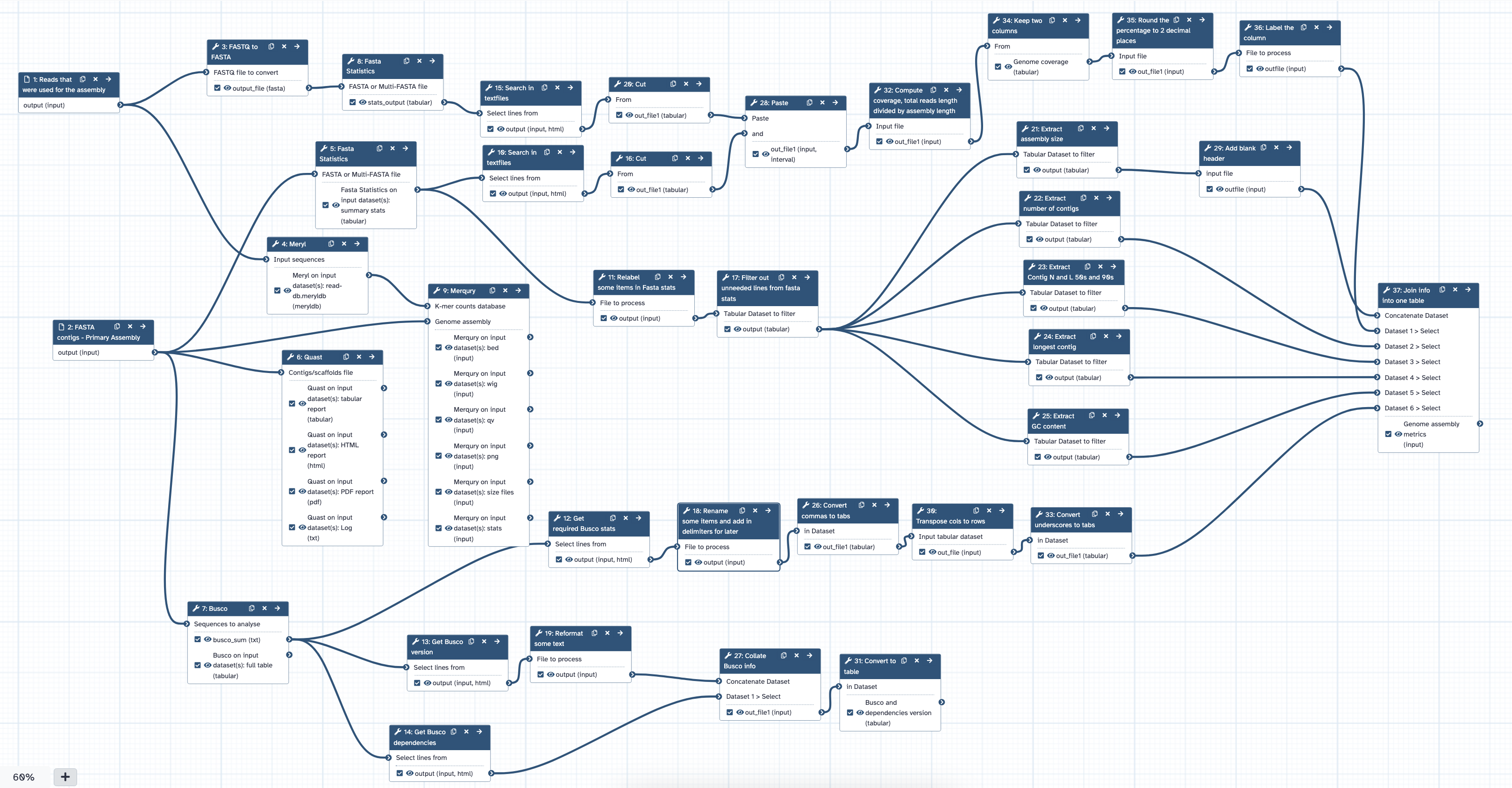
Fig 1. The Genome assessment post assembly workflow.
Once you have checked the genome assembly, you may decide that:
- Further sequencing is required (e.g. sequencing depth was not sufficient for genome size)
- The assembly should be repeated with different parameters (e.g. to improve contiguity)
- The genome assembly is good enough to proceed.
How to cite the workflow
Kate Farquharson, Gareth Price, Simon Tang, Anna Syme (2024). Genome-assessment-post-assembly. WorkflowHub. https://doi.org/10.48546/WORKFLOWHUB.WORKFLOW.403.7
A note on software versions
| Software | Version |
|---|---|
| FASTA stats | 2.0 |
| QUAST | 5.0.2+galaxy1 |
| BUSCO | 5.4.6+galaxy0 |
| Meryl | 1.3+galaxy6 |
| Merqury | 1.3 |
Standards of genome quality
Note that there is no such thing as the perfect genome! Standards such as the Earth BioGenome Project’s Table of Proposed EBP Metrics can be used as a guide for genome quality, noting that these standards rely on a scaffolded (e.g. HiC) genome (Rhie et al. below)
Rhie, A., McCarthy, S.A., Fedrigo, O. et al. Towards complete and error-free genome assemblies of all vertebrate species. Nature 592, 737–746 (2021). https://doi.org/10.1038/s41586-021-03451-0
| Tool or workflow | EBP metric provided (Rhie et al. 2021) |
|---|---|
| Merqury | False duplications - Base pair QV - K-mer completeness - Phased block (NG50) |
| Purge duplicates | Curation improvements - false duplication removal |
| BUSCO | Genes |
Before you start!
The QC workflow
- Is optimised for assessment of eukaryotic genomes. It can be reconfigured for prokaryotic or fungal genomes.
This How-to-Guide
- Covers how to analyse a single genome.
- If you had access to sequence data for trios and wanted to calculate things like phase block continuity, please to refer to the Merqury documentation.
Genome assessment post assembly workflow
- Make sure you are registered and logged into Galaxy Australia
- Upload your primary genome assembly file and the reads that were used in the genome assembly, i.e. the filtered reads (concatenate multiple read files into a single file) to your current Galaxy history
- Note that the reads should be in the format
fastqsanger.gz - If you are coming to this workflow after the hifiasm assembly workflow, you will need to convert the reads (that have had adapters removed) from
fastq.gztofastqsanger.gz - Click on the pencil icon near the file name, go to Datatypes, Assign Datatype, and assign a new Datatype
- If you are coming to this workflow after the nanopore assembly workflow, you will need to convert the reads (from Nanofilt) from
fastqsangertofastqsanger.gz - Click on the pencil icon near the file name, go to Datatypes, Convert to Datatype, and choose the compressed file
- See this link for details on how to upload files
- If you don’t have a history (i.e. you are using an existing assembly), you can create one (click the plus button at the top of this history panel).
- Note that the reads should be in the format
-
Visit this link to:
- retrieve the workflow for assembly quality control,
- add it to your Galaxy Australia workflows list, and
- open your workflows list (which can also be reached by clicking the
Workflowtab), highlighted by a red box in Fig 3) - the URL for this tab is https://usegalaxy.org.au/workflows/list

Fig 3. The main page of the Galaxy Australia service.
- Select the play button (highlighted by a red box in Fig 4) for the
Genome assessment post assemblyworkflow.
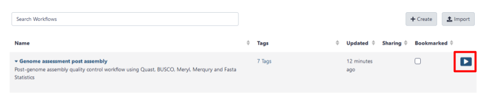
Fig 4. The workflows page of the Galaxy Australia service is where your workflows appear. The play button to launch your workflow is highlighted by a red box.
Edit from the drop down menu.-
The workflow invocation window will open. Click
-
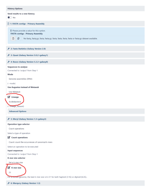
Select input data for the assembly. Choose either the primary assembly file that you previously loaded into your Galaxy history, or the assembly you created using the Galaxy HiFi genome assembly workflow, using the drop-down menu (step 1 in Fig 5). The genome assembly should be in
fastaformat.
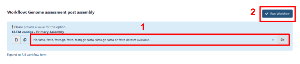
Fig 5. The workflow invocation menu for the Genome assessment post assembly workflow. Step 1 is to select the primary assembly file using the drop-down menu, and Step 2 is to select Run workflow.
-
Select input data for the sequencing reads. These should be the HiFi or Nanopore reads, that have had adapters removed, and then concatenated into a single file. This should be in
fastqsanger.gzformat. -
Determine optimal k-mer size for genome
- In order for Meryl to generate a database for each read file, a k-mer length must be selected
- It should be large enough to allow the k-mer to map uniquely to the genome
- k = 21 is generally a good length for a haploid genome of 3.1 Gb and a diploid genome of 6.2 Gb
-
BUSCO lineage selection
- In this workflow, the default setting for lineage is
eukaryota - However, you can select an alternative lineage relevant to your genome
- For example, if you were analysing a lizard genome, you may wish to select the Sauropsida lineage
- Alternatively, you may prefer to select a broader lineage such as Vertebrata to allow for broader comparisons to other species’ genomes
- Keeping in mind that BUSCO results should generally be compared across the same version of BUSCO and the same lineage
- In this workflow, the default setting for lineage is
-
Quast settings
- In this workflow, the default setting for lineage is
eukaryotes - However, you can select an alternative lineage relevant to your genome
- In this workflow, the default setting for
Is genome large (>100 Mbp)?isyes, but this can be changed
- In this workflow, the default setting for lineage is
- Click
Run workflow(step 2 in Fig 5).
Genome assessment workflow outputs
Below are descriptions of the workflow outputs, including those for FASTA statistics, the QUAST report (webpage, PDF and tabular*), BUSCO and Merqury. A more in-depth Merqury guide is also available below.
FASTA statistics
Kyran, A. (2021). Fasta Statistics: Display summary statistics for a fasta file. https://github.com/galaxyproject/tools-iuc
A general QC tool for FASTA files, which produces a summary table (see Fig 6).
The metrics include various sequence read lengths (n50, min, max, median and average),
numbers of base pairs (A, C, G, T, N, total number num_bp and total number that are not N num_bp_not_N),
the total number of sequences as well as the GC content.
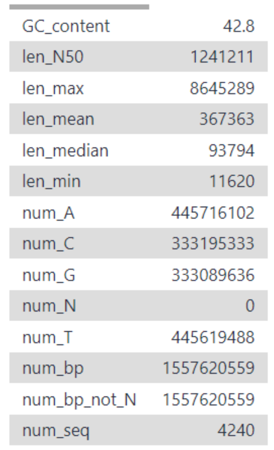
Fig 6. FASTA statistics output
num_bp)
is similar to what you expected based on other related genomes (noting that for some taxa,
there is substantial variation in genome size across taxa).QUAST report
https://bio.tools/quast & Gurevich, A., Saveliev, V., Vyahhi, N., & Tesler, G. (2013). QUAST: quality assessment tool for genome assemblies. Bioinformatics, 29(8), 1072–1075. https://doi.org/10.1093/bioinformatics/btt086
QUAST returns a number of metrics assessing genome quality. In particular, note some commonly reported metrics:
- No. contigs: total number of contigs in the assembly (i.e. how many pieces the genome is in). The lower the number of contigs, the less fragmented the genome.
- N50: the length at which all contigs of that length or longer cover at least half of the assembly. The higher the N50, the better.
- L50: the number of contigs equal to or longer than N50 (i.e. the minimal number of contigs that cover half the assembly). The lower the L50, the better.
See the QUAST user guide for additional detail.
The most useful QUAST output is likely to be the summary report in either .txt, .pdf or .html format.
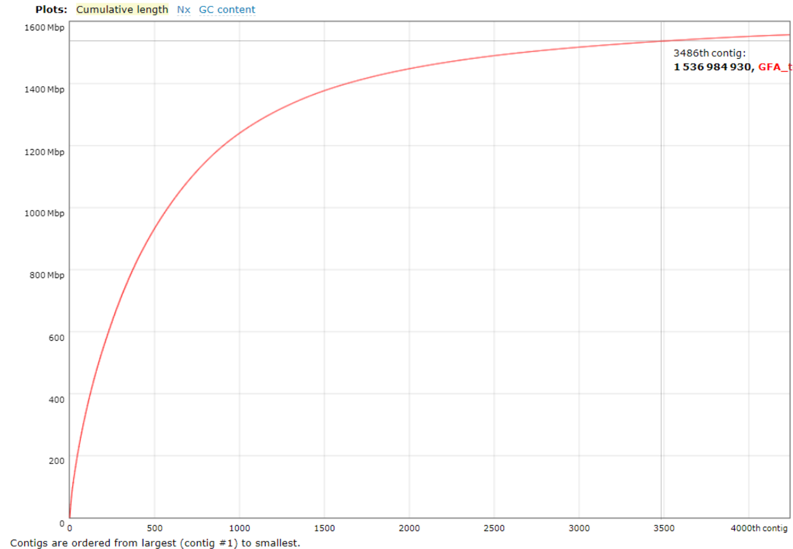
Fig 7. QUAST output PDF
BUSCO
https://bio.tools/busco & Simão, F. A., Waterhouse, R. M., Ioannidis, P., Kriventseva, E. V., & Zdobnov, E. M. (2015). BUSCO: assessing genome assembly and annotation completeness with single-copy orthologs. Bioinformatics, 31(19), 3210–3212. https://doi.org/10.1093/bioinformatics/btv351
BUSCO (Benchmarking Universal Single-Copy Orthologs) is a tool used to measure “completeness” of a genome by comparing the assembly to a selected “lineage” of evolutionarily conserved single-copy genes. Because the genes are evolutionarily conserved, we expect that they should be found once in the genome assembly. The BUSCO results show the number and % of all BUSCOs that were identified in the assembly as either complete (broken down by either single-copy or duplicated form), fragmented, or missing (i.e. not present in the assembly).
Higher complete single-copy BUSCO scores are generally considered better. However, the BUSCO score can be impacted by the lineage used (e.g. for a skink, you could select vertebrata, tetrapoda or the squamata lineages), the divergence of the species to the reference lineage, and the assembly quality.
If reporting BUSCO in a publication, be sure to report the:
- version of BUSCO used,
- lineage dataset selected,
- number of BUSCOs in the lineage, and
- full score
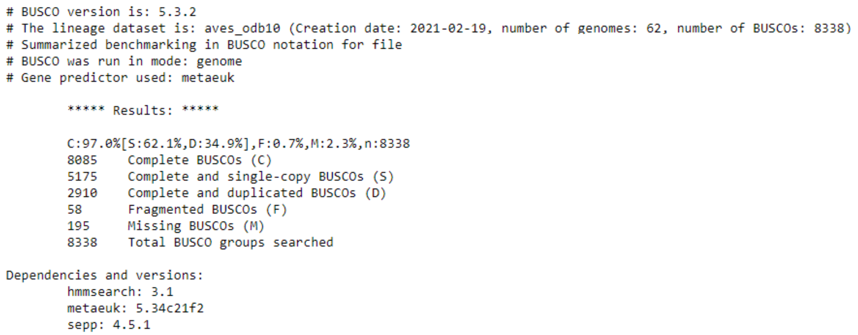
Fig 8. Example BUSCO output
Merqury & meryl
Meryl produces a meryldb (download only, no visualisation available), which is required for Merqury. It is visible in the workflow to allow for easy access, and to allow input for tools other than Merqury
Additional tables
Two additional tables are created and displayed as output files, as well as in the workflow report.
These are:
- a table for assembly statistics, which includes a calculation of genome coverage and selected lines from the Fasta Statistics output
- a table to show the version of BUSCO and its dependencies
PacBio HiFi Single Genome Assessment with merqury
Introduction: What is merqury, and what can it be used for?
Merqury is used to evaluate de novo genome assemblies. It works by comparing pre-defined k-mers in unassembled, high accuracy reads with the assembled genome, and then calculates metrics like the base-level accuracy and completeness based on these statistics. Unlike other evaluation tools such as BUSCO, it is reference-free, and thus is not vulnerable to problems like true copy number variants in genes.
Analysing Output Files and Viewing Images
Several files will be generated. Below, the main files relevant for genome assessments are described and what their outputs mean.
output.completeness.stats
This records the k-mer completeness - the metric (%) is calculated as the fraction of reliable k-mers in the read set that are also found in the assembly. The number of these k-mers is mathematically calculated from the spectra-cn plots (seen in images below). The equation for the slope of the histogram is calculated, and the first instance of a positive slope is the threshold point for reliable k-mers (all k-mers following from this threshold are reliably incorporated into the genome with low sequencing errors). This is likely a quality statistic that should be recorded in a publication as it assesses how complete the genome is - the more k-mers in the reads set that end up in the assembly, the more informed the genome is, and thus the better.
Column descriptors are below, with some sample results generated from test data used in the Merqury publication (A. thaliana dataset):
|Assembly name|k-mer set used (all = reads set)|solid k-mers in the assembly|total solid k-mers in the read set|Completeness (%)| |:—:|:—:|:—:|:—:|:—:| |athal_COL|all|104975080|125303808|83.7764| Source of table data: https://github.com/marbl/merqury
Command used to generate results: $MERQURY/merqury.sh F1.k18.meryl athal_COL.fasta test-1
output_merqury.completeness
The columns in this output are:
- Assembly
- k-mer set used for measuring completeness -
all= read set (this gets expended with hap-mers later) - Solid k-mers in the assembly
- Total solid k-mers in the read set
- Completeness (%)
Information source: https://github.com/marbl/merqury/wiki/2.-Overall-k-mer-evaluation
output_merqury
The columns in this output are:
- Assembly of interest. Both is combined of the above two.
- k-mers uniquely found only in the assembly
- k-mers found in both assembly and the read set
- QV (consensus quality value)
- Error rate
output.qv
This is the consensus quality of the genome. QV is a assembly quality metric, based on the number of k-mers that are found only in the assembly but not in the reads (which would imply consensus base pair errors). To calculate this, the error rate is first determined. The proportion of unique k-mers in the assembly over the total number of k-mers in the assembly represent the error rate, as they are assumed to have base errors. Then, it is recorded as a log-scaled probability of error for the consensus base calls (Phred Quality Score). See below the calculation for QV, with E being error rate.
QV = −10log E
Q30 corresponds to 99.90% accuracy, Q40 to 99.99%, etc.
Column descriptors are below, with sample data from the same A. thaliana dataset:
| Assembly name | k-mers found only in assembly | k-mers found in both assembly and reads | QV | Error rate (E) |
|---|---|---|---|---|
| athal_COL | 682359 | 123511626 | 35.1183 | 0.000307729 |
The above output makes the claim that the assembly is 99.90 - 99.99% accurate.
output.genome.qv
This is the consensus quality of each individual contig. There isn’t too much value with many contigs, and serves more as a diagnostic tool to see any potential contig outliers. It follows a similar format to the whole genome QV. See below some sample results from the A. thaliana dataset:
| Contig name | k-mers from contig found only in assembly | k-mers from contig found in both assembly and reads | QV | Error rate |
|---|---|---|---|---|
| tig00000032 | 1718 | 3789945 | 45.9879 | 2.5189e-05 |
| tig00000159 | 2744 | 3634845 | 43.7722 | 4.19547e-05 |
genome_only.bed
This file is provided to trace the bp errors. This is useful for finding mis-assembly sites, which usually involves low bp
quality region. It is basically a .bed representation of the k-mers generated from each read.
genome_only.wig
This file is provided to trace the bp errors. This is useful for finding mis-assembly sites, which usually involves low bp quality region. It is basically a .wig representation of the k-mers generated from each read.
Images
The images are histograms that represent different things (note that ln means histogram represented by just lines, fl means histogram is filled in, and st means histogram is stacked).
output.genome.spectra-cn.<fl/ln/st>.png
These are spectra-cn plots, which record the copy number of k-mers. ‘k-mer multiplicity’ records the number of times a certain k-mer appears in the reads, and ‘Count’ records the number of k-mers that have appeared that number of times. For example, in the graph below, about 3.9 x 10^6 k-mers appeared 45 times in the reads.
The different colours relate to the number of times the k-mer appears in the genome assembly itself. 2-copy k-mers are present in both haplotypes (homozygosity) and 1-copy k-mers are present in only one haplotype (and thus represent heterozygosity). Grey represents the k-mers found only in the reads (not assembled into the genome) and the small bar of red and blue on the left represent k-mers only found in the assembly (sequencing error).
This is a great graph to include in a publication as it provides both an accurate k-mer distribution of your genome, but also extra information about the heterozygosity and sequencing errors.
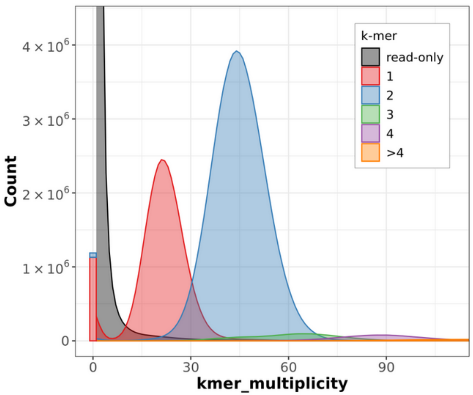
Fig 9. Merqury output.genome.spectra-cn output
output.spectra-asm.<fl/ln/st>.png
This is relevant when you are looking at trios or comparing parental genomes - this shows the proportion of k-mers that are shared between them. No need to look at these for single genome analysis.
Affiliations

 Editor
Australian BioCommons, University of Melbourne
