Run nf-core/proteinfold on Setonix
Overview
Teaching: 5 min
Exercises: 15 minQuestions
Objectives
Run nfcore/proteinfold Nextflow workflow on Setonix.
Monitor resource allocation and utilisation.
Evaluate the cost of execution.
Prepare samplesheet
We have prepared a Nextflow samplesheet containing our protein input in FASTA format.
Each prediction must be given a unique id and an input file containing the target sequence
cat samplesheet.csv
Output:
id,fasta
sample0,fasta/PNK_0205.fasta
Standard run
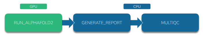
This is the structure of a standard proteinfold workflow execution:
-
Execute the workflow using the script below:
 nextflow run nf-core/proteinfold/ \
     --input samplesheet.csv \
     --outdir output/ \
     --db /scratch/references/abacbs2025/databases/ \
     --mode alphafold2 \
     --use_gpu \
     --alphafold2_mode "standard" \
     -c abacbs_profile.config \
     --slurm_account $PAWSEY_PROJECT \
     -r 53a1008
Note
Make sure you have loaded the required modules and set the neccessary environment variables from the earlier episodes in this terminal.
Job monitoring
-
Open a new VScode terminal using the
+in the top-right corner of the terminal panel.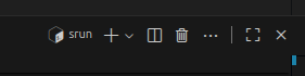
-
In our second terminal we can confirm that our job is running with:
squeue --meJOBID USER ACCOUNT NAME EXEC_HOST ST REASON START_TIME END_TIME TIME_LEFT NODES PRIORITY QOS 34776177 tlitfin pawsey1017-gpu nf-NFCORE_PROT nid002166 R None 08:15:36 20:15:36 11:36:58 1 75399 normal -
Similarly, we can connect to the node that is executing the job to check the status (ie the node id under EXEC_HOST). Replace
with the id under EXEC_HOST (eg nid002166 from the example above). ssh <node> -
Type
yeswhen prompted and then enter your workshop account password at the password prompt. Note: you can only connect to nodes where you have an active job runningwatch rocm-smi -
We can monitor GPU utilization in the last column:
 ========================================= ROCm System Management Interface =========================================
 =================================================== Concise Info ===================================================
 Device  Node  IDs              Temp    Power  Partitions          SCLK    MCLK     Fan  Perf  PwrCap  VRAM%  GPU%
 ^[3m              (DID,     GUID)  (Edge)  (Avg)  (Mem, Compute, ID)                                                   ^[0m
 ====================================================================================================================
 0       11    0x7408,   49174  35.0°C  N/A    N/A, N/A, 0         800Mhz  1600Mhz  0%   auto  0.0W    74%    0%
 ====================================================================================================================
 =============================================== End of ROCm SMI Log ================================================
Job Accounting
-
After the workflow has completed, view the
execution_timelineHTML file located in theoutput/pipeline_info/directory. -
You can find the file by navigating to the
exercises/exercise2/output/pipeline_info/directory in theVSCodefile browser in the left-hand panel -
Right-click the
execution_timelinefile and selectPreview.
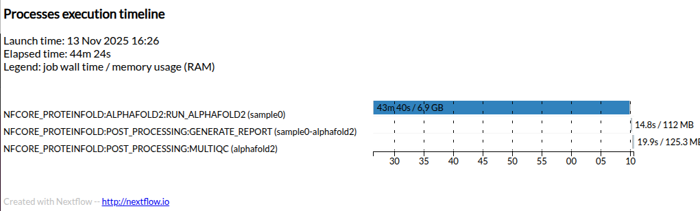
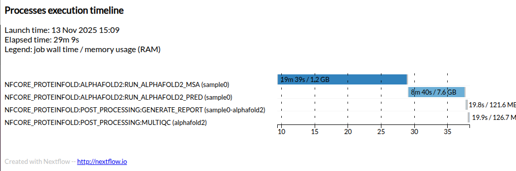
Execution timeline
Here is an example timeline from a full AlphaFold2 run for this target protein.
Your execution time will be greatly reduced by using dummy miniature databases and generating only a single AlphaFold2 model output.
Service units
- All Pawsey users are allocated service units (SU) which are consumed by running jobs on Setonix.
- The SU cost of each job is determined based on the requested resources.
- We can use the Pawsey calculator to estimate the SU cost of our workflow execution.
- A full scale execution was completed in 0.75 hours using a single GPU (neglible CPU time).
Calculation Breakdown
SUs = Partition Charge Rate × Max Proportion × Nodes × Hours
512 × 0.1250 × 1 × 0.75 = 48 SUs
GPU Proportion: 1 GCDs / 8 total GCDs = 0.1250
- Compare this with the execution time for the demo run from this workshow using the miniature databases.
A basic run of AlphaFold2 for this target using the official implementation consumes 48 SUs on the Setonix system.
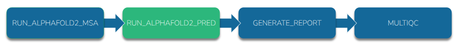
Split MSA run
Recall that AlphaFold2 relies on generating an MSA by searching large sequence databases.
This search process does not invoke the GPU which means that it is wasteful to request a GPU node until the MSA has been generated.
We can split AlphaFold2 into a part that requires the CPU and a part that requires the GPU. Nextflow can send jobs to the appropriate resource.
-
Re-run proteinfold to predict the same protein but this time use AlphaFold2 in
"split_msa_prediction"mode:nextflow run nf-core/proteinfold \ --input samplesheet.csv \ --outdir output-split/ \ --db /scratch/references/abacbs2025/databases/ \ --mode alphafold2 \ --use_gpu \ --alphafold2_mode "split_msa_prediction" \ -c abacbs_profile.config \ --slurm_account $PAWSEY_PROJECT \ -r 53a1008
Note
Make sure you have loaded the required modules and set the neccessary environment variables from the earlier episodes in this terminal.
Job Accounting
-
After the workflow has completed, view the
execution_timelineHTML file located in theoutput-split/pipeline_info/directory. -
You can find the file by navigating to the
exercises/exercise2/output/pipeline_info/directory in theVSCodefile browser in the left-hand panel -
Right-click the
execution_timelinefile and selectPreview.
Execution timeline
Here is an example timeline from a full AlphaFold2 run using
"split_msa_prediction"for this target protein.Your execution time will be greatly reduced by using dummy miniature databases and generating only a single AlphaFold2 model output.
Service units
We can again use the Pawsey calculator to estimate the service unit (SU) cost.
A full scale execution was completed in 0.16 hours using a single GPU and 0.3 hours of CPU time.
CPU
SUs = Partition Charge Rate × Max Proportion × Nodes × Hours
128 × 0.0696 × 1 × 0.3 = 2.672 SUs

Core Proportion: 8 cores / 128 total cores = 0.0625
Memory Proportion: 16 GB / 230 GB total for accounting = 0.0696
Max Proportion (Memory): 0.0696
GPUSUs = Partition Charge Rate × Max Proportion × Nodes × Hours 512 × 0.1250 × 1 × 0.16 = 10.24 SUs GPU Proportion: 1 GCDs / 8 total GCDs = 0.1250Compare the SU cost of running all work on a GPU node compared with splitting the job to more efficiently use the appropriate resource.
Standard:               48   SUs
Split MSA: 2.7 + 10.2 = 12.9 SUs
By splitting the MSA step to a CPU node, we can run AlphaFold2 for this target using ~13 SUs (compared with 48 SUs for the original run) on the Setonix system.
Note
To minimise idle GPU time, it is important to ensure CPU-bound work is sent to a CPU node. This can lead to big savings in SU allocation!
Key Points
Nextflow can be used to orchestrate AlphaFold2 executions.
We can monitor resource utilisation by connecting to a worker node.
Running AlphaFold2 in split mode can significantly reduce SU consumption.